Experiment 2: RDK Direction Judgement, 4 Tasks, 500 msec Error Penalty
knowlabUnimelb
2020-10-29
Last updated: 2025-07-29
Checks: 7 0
Knit directory: SCHEDULING/
This reproducible R Markdown analysis was created with workflowr (version 1.7.1). The Checks tab describes the reproducibility checks that were applied when the results were created. The Past versions tab lists the development history.
Great! Since the R Markdown file has been committed to the Git repository, you know the exact version of the code that produced these results.
Great job! The global environment was empty. Objects defined in the global environment can affect the analysis in your R Markdown file in unknown ways. For reproduciblity it’s best to always run the code in an empty environment.
The command set.seed(20221107) was run prior to running
the code in the R Markdown file. Setting a seed ensures that any results
that rely on randomness, e.g. subsampling or permutations, are
reproducible.
Great job! Recording the operating system, R version, and package versions is critical for reproducibility.
Nice! There were no cached chunks for this analysis, so you can be confident that you successfully produced the results during this run.
Great job! Using relative paths to the files within your workflowr project makes it easier to run your code on other machines.
Great! You are using Git for version control. Tracking code development and connecting the code version to the results is critical for reproducibility.
The results in this page were generated with repository version 2c1fd06. See the Past versions tab to see a history of the changes made to the R Markdown and HTML files.
Note that you need to be careful to ensure that all relevant files for
the analysis have been committed to Git prior to generating the results
(you can use wflow_publish or
wflow_git_commit). workflowr only checks the R Markdown
file, but you know if there are other scripts or data files that it
depends on. Below is the status of the Git repository when the results
were generated:
Ignored files:
    Ignored:    .Rhistory
    Ignored:    .Rproj.user/
    Ignored:    analysis/patch_selection.png
    Ignored:    analysis/patch_selection_8.png
    Ignored:    analysis/patch_selection_avg.png
    Ignored:    analysis/site_libs/

Untracked files:
    Untracked:  analysis/Notes.txt
    Untracked:  analysis/additional_scripts.R
    Untracked:  analysis/analysis_2025_deadlines.Rmd
    Untracked:  analysis/analysis_2025_dynamicNoise_fixed.Rmd
    Untracked:  analysis/analysis_exp10_preemption.Rmd
    Untracked:  analysis/analysis_exp10_preemption1and2.Rmd
    Untracked:  analysis/analysis_exp10b_preemption-pareto.Rmd
    Untracked:  analysis/analysis_exp11_facesInNoise.Rmd
    Untracked:  analysis/analysis_exp11_facesInNoise_EW.Rmd
    Untracked:  analysis/analysis_exp11_facesInNoise_EW_v2.Rmd
    Untracked:  analysis/analysis_exp12_variability.Rmd
    Untracked:  analysis/analysis_exp12_variability_cynthia.Rmd
    Untracked:  analysis/analysis_exp12_variability_cynthia_update.Rmd
    Untracked:  analysis/analysis_exp13_preemption.Rmd
    Untracked:  analysis/analysis_exp14_ASD_individual_differences.Rmd
    Untracked:  analysis/analysis_exp9_preselection.Rmd
    Untracked:  analysis/analysis_exp9_preselection1and2.Rmd
    Untracked:  analysis/analysis_exp9_select-then-complete.Rmd
    Untracked:  analysis/anovaData/
    Untracked:  analysis/archive/
    Untracked:  analysis/correlation_test.m
    Untracked:  analysis/fd_pl.rds
    Untracked:  analysis/fu_pl.rds
    Untracked:  analysis/instructions_for_honours_students.txt
    Untracked:  analysis/joyPlot.m
    Untracked:  analysis/joyPlot.zip
    Untracked:  analysis/joyPlot/
    Untracked:  analysis/loadData.m
    Untracked:  analysis/mstrfind.m
    Untracked:  analysis/plotDistanceByTrials.m
    Untracked:  analysis/prereg/
    Untracked:  analysis/reward rate analysis.docx
    Untracked:  analysis/rewardRate.jpg
    Untracked:  analysis/scheduling_analysis_functions.R
    Untracked:  analysis/temp/
    Untracked:  analysis/toAnalyse/
    Untracked:  analysis/wflow_code_string.txt
    Untracked:  code/AUTSIMQ/
    Untracked:  code/DYNAMICNOISE/
    Untracked:  code/FACESINNOISE/
    Untracked:  code/Notes on how the scheduling jsPsych code works.txt
    Untracked:  code/PREEMPT/
    Untracked:  code/PREPLAN/
    Untracked:  code/SCHEDULEPIX/
    Untracked:  code/SCHEDULEPIX_UON/
    Untracked:  code/SCHEDULERDK/
    Untracked:  code/SCHEDULERDK_UON/
    Untracked:  code/SCHEDULE_REWARD/
    Untracked:  code/SCHEDULE_TYPING/
    Untracked:  code/SMALL_N_LETTERNOISE/
    Untracked:  code/TRAIN_PREEMPT/
    Untracked:  code/TRAIN_VARYING_DEADLINES/
    Untracked:  code/autism_quotient.txt
    Untracked:  data/2020_exp1_rdk_data.csv
    Untracked:  data/2020_exp2_rdk_data.csv
    Untracked:  data/2021_exp2b_rdk_data_avgtime.csv
    Untracked:  data/2023-exp10-preemption-pareto.csv
    Untracked:  data/2023-exp10-preemption-selections.csv
    Untracked:  data/2023-exp10-preemption.csv
    Untracked:  data/2023-exp11-facesInNoise-unlabelledCondition.csv
    Untracked:  data/2023-exp11-facesInNoise.csv
    Untracked:  data/2023-exp9-preplan.csv
    Untracked:  data/2023-exp9-select-then-complete.csv
    Untracked:  data/2023_AQdata.csv
    Untracked:  data/2024-exp12-variability.csv
    Untracked:  data/2024-exp12-variability_v2.csv
    Untracked:  data/2024-exp12-variability_v3.csv
    Untracked:  data/2024-exp13-preemption.csv
    Untracked:  data/2024-exp13-preemption_v2.csv
    Untracked:  data/2024-scheduling-data.csv
    Untracked:  data/2024_data_rdk_select_first_AQcorrelation_update.csv
    Untracked:  data/2024_data_typing_train_variability.csv
    Untracked:  data/2025_data_dynamic_noise_fixed_locations.csv
    Untracked:  data/2025_data_typing_train_deadlines_exp1rates.csv
    Untracked:  data/2025_data_typing_train_variability_fulldataset.csv
    Untracked:  data/ASRSscoring.csv
    Untracked:  data/OLIFEscoring.csv
    Untracked:  data/OLIFEscoring_v0.csv
    Untracked:  data/POLYscoring.csv
    Untracked:  data/SQL query.txt
    Untracked:  data/archive/
    Untracked:  data/create_database.sql
    Untracked:  data/dataToAnalyse/
    Untracked:  data/data_dictionary_deadlines.csv
    Untracked:  data/data_dictionary_dynamic_noise.csv
    Untracked:  data/data_dictionary_facesInNoise.csv
    Untracked:  data/data_dictionary_preemption.csv
    Untracked:  data/data_dictionary_preplan.csv
    Untracked:  data/data_dictionary_select_then_complete.csv
    Untracked:  data/data_dictionary_variability.csv
    Untracked:  data/exp3a_rdk_data_dynamic_selections.csv
    Untracked:  data/exp3b_rdk_data_dynamic_highlight_selections.csv
    Untracked:  data/exp6a_typing_exponential.xlsx
    Untracked:  data/exp6b_typing_linear.xlsx
    Untracked:  data/exp8a_typing_no_reward_data_selections.csv
    Untracked:  data/rawdata_incEmails/
    Untracked:  data/selections/
    Untracked:  data/sona data/
    Untracked:  data/summaryFiles/
    Untracked:  data/temp_AQcorrelationReplication/
    Untracked:  spatial_pdist.Rdata

Unstaged changes:
    Modified:   analysis/analysis_exp1_labelled_nodelay.Rmd
    Modified:   analysis/analysis_exp3a_rdk_dynamic_delay.Rmd
    Modified:   analysis/analysis_exp3b_rdk_dynamic_delay_highlight.Rmd
    Modified:   analysis/analysis_exp7e_rdk_reward_points.Rmd
    Modified:   analysis/analysis_exp8a_typing_no_reward.Rmd
    Deleted:    analysis/prereg.Rmd
    Deleted:    analysis/prereg_v2.Rmd
    Deleted:    analysis/prereg_v3.Rmd
    Deleted:    analysis/prereg_v6_AQcorrelation.Rmd
    Modified:   data/README.md
    Modified:   data/data_dictionary.csv
    Modified:   data/data_dictionary_avgTime.csv
    Modified:   data/data_dictionary_ruby.csv
    Deleted:    data/exp1_rdk_data.csv
    Deleted:    data/exp2_rdk_data.csv
    Deleted:    data/exp2b_rdk_data_avgtime.csv
Note that any generated files, e.g. HTML, png, CSS, etc., are not included in this status report because it is ok for generated content to have uncommitted changes.
These are the previous versions of the repository in which changes were
made to the R Markdown
(analysis/analysis_exp2a_labelled_delay.Rmd) and HTML
(docs/analysis_exp2a_labelled_delay.html) files. If you’ve
configured a remote Git repository (see ?wflow_git_remote),
click on the hyperlinks in the table below to view the files as they
were in that past version.
| File | Version | Author | Date | Message |
|---|---|---|---|---|
| Rmd | 2c1fd06 | knowlabUnimelb | 2025-07-29 | Fix markdown in 2a and update analysis code to use shared file repo in 2b |
| html | 22ddfa1 | knowlabUnimelb | 2025-07-29 | Build site. |
| Rmd | 73c8f5b | knowlabUnimelb | 2025-07-29 | Update analysis code to use shared file repo |
| html | 2e6ecdf | knowlabUnimelb | 2022-11-09 | Build site. |
| Rmd | 67e1aac | knowlabUnimelb | 2022-11-09 | Publish data and analysis files |
Daniel R. Little1, Ami Eidels2 1 The University of Melbourne, 2 The University of Newcastle
Method
Participants
We tested 100 participants (90 F, 9 M, 1 Undeclared). Participants were recruited through the Melbourne School of Psychological Sciences Research Experience Pool (Mean age = 19.25, range = 17 - 40). Participants were reimbursed with credit toward completion of a first-year psychology subject.
were assigned to the Fixed Difficulty condition. In this condition, the location of easy, medium, hard, and very hard random dot kinematograms (RDK’s) was held constant across trials.
were assigned to the Random Difficulty condition. In this condition, the location of easy, medium, hard, and very hard random dot kinematograms (RDK’s) were randomized from trial to trial.
The Fixed Difficulty experiment was completed before the Random Difficulty experiment. Participants only completed one of these.
Design
In each condition, participants completed multiple trials in which they selected and completed RDK tasks. On each trial, participants were shown a set of four RDKs labelled Easy, Medium, Hard, and Very Hard. The labels corresponded to the coherence of the RDK; that is, the proportion of dots moving in a coherent direction was set to 80%, 50%, 20%, and 0% for the Easy, Medium, Hard, and Very Hard locations, respectively. From the set of four RDKs, participants selected and completed one RDK at a time in any order. The goal of each trial was to complete as many as possible before a deadline. If an incorrect RDK response was made, that RDK was restarted at the same coherence but with a resampled direction (so the direction may have changed), and the participant had to respond to the RDK again. A new task could not be selected until the RDK was completed successfully.
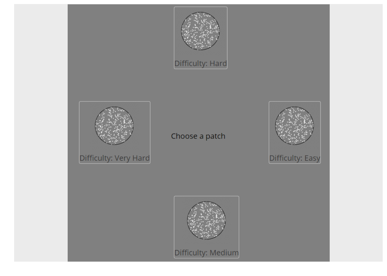
Participants first completed 10 trials with a long (30 sec) deadline to help participants learn the task, explore strategies, and allow for comparison to a short-deadline condition. We term this the no deadline condition since the provided time is well beyond what is necessary to complete all four RDK’s. Next, participants completed 30 trials with a 6 second deadline.
Data Cleaning
Subjects completed the experiment by clicking a link with the uniquely generated id code. Subjects were able to use the link multiple times; further, subjects were able to exit the experiment at any time. Consequently, the datafile contains partially completed data for some subjects which needed to be identified and removed.
After removing any participants who had less than chance accuracy on the easiest RDK indicating equipment problems or a misunderstanding of task directions, there were 47 and 50 in the fixed and random location conditions, respectively.
Data Analysis
We first summarize performance by answering the following questions:
Task completions
- How many tasks are completed on average?
Across both conditions, participants completed 3.88 tasks during the untimed phase and 3.3 tasks during the deadline phase.
RDK performance
We next analysed performance on the RDK discriminations. We then asked:
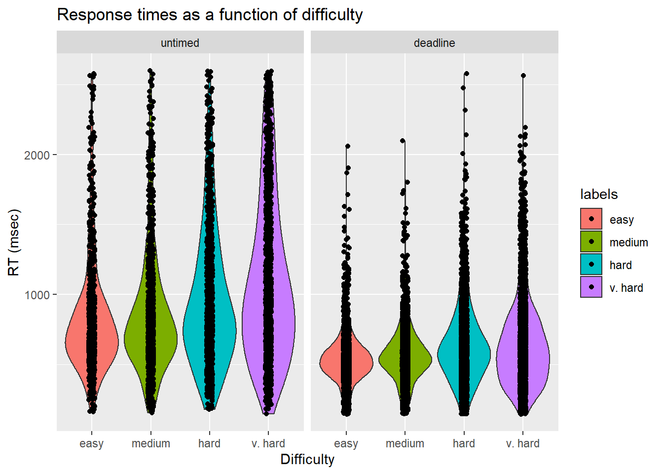
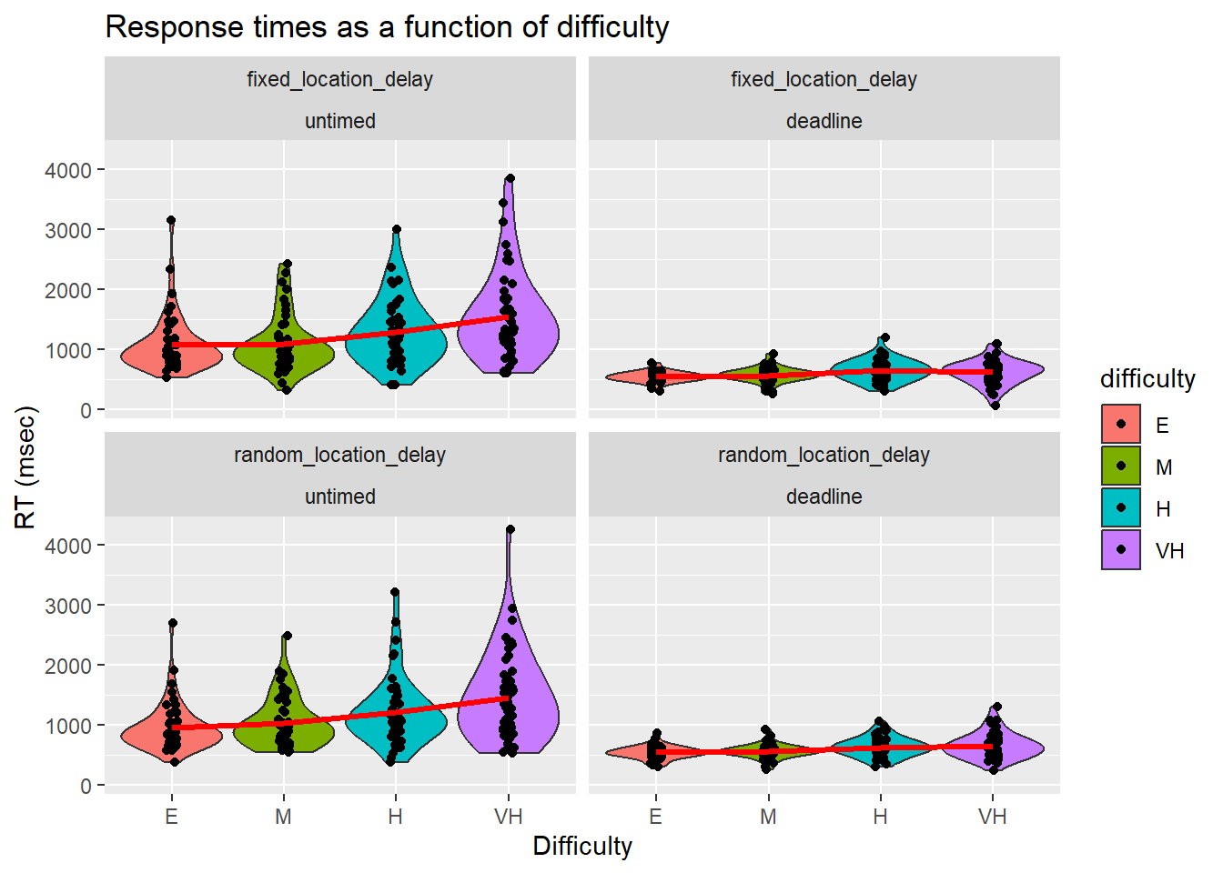
- What was the average completion time and accuracy of the easy, medium, hard, and very hard tasks?
RTs became shorter and more accurate as the difficulty of the RDK became easier. As expected, the RTs were shorter under a deadline than without a deadline. We visualised the response times in two ways: First, we simply took the average of each attempt on each RDK.
| Version | Author | Date |
|---|---|---|
| 22ddfa1 | knowlabUnimelb | 2025-07-29 |
| Version | Author | Date |
|---|---|---|
| 22ddfa1 | knowlabUnimelb | 2025-07-29 |
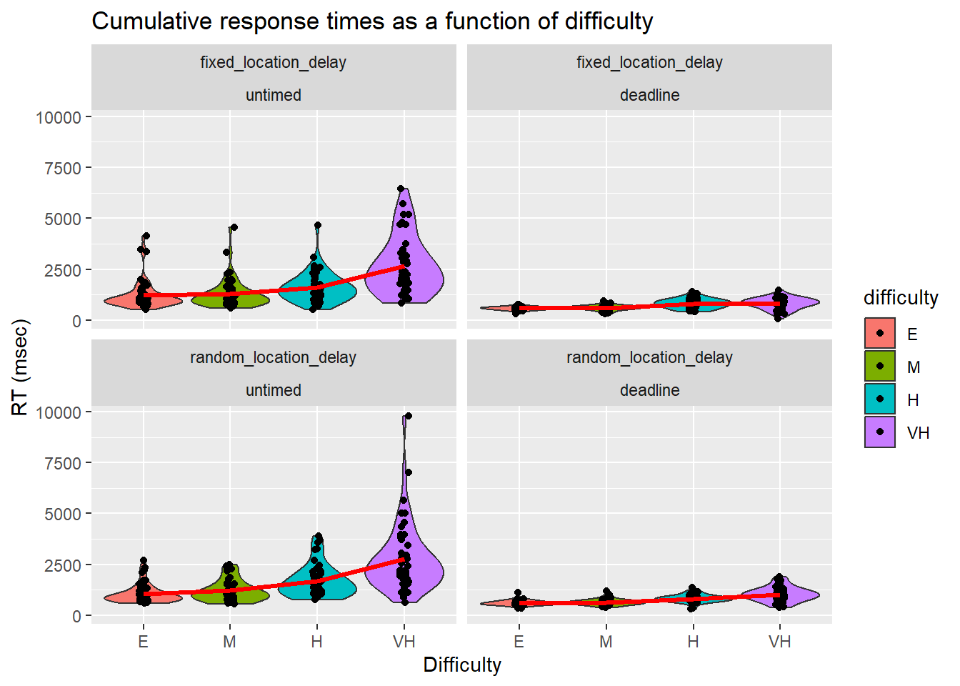
Second, we computed the time to complete an RDK as the cumulative sum across multiple attempts within a trial (termed Cumulative RT or cRT). That is, if an error is made and the RDK needs to be repeated, then the total RT is the sum of both attempts.
We further broke down RTs by condition, deadline, and difficulty.
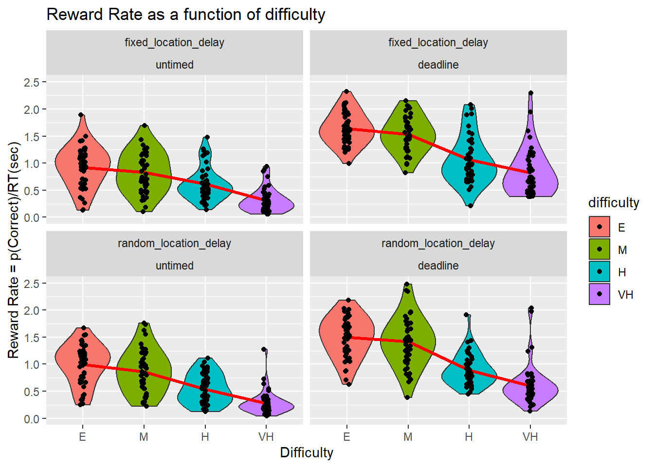
Reward Rate
To confirm that coherence offered a good proxy for difficulty (and hence, that an optimal order of easiest to hardest was maintained), we calculated the reward rate for each patch. Reward rate can be defined as “the proportion of correct trials divided by the average duration between decisions” (Gold & Shadlen, 2002), and is tantamount, in our task, to percentage of correct responses per unit time (Bogacz et al, 2006). For our purposes, we can fix time at 1 sec calculate the Reward Rate as the number of RDK tasks completed in 1 sec.
Inspection of the figure reveals that RR is roughly monotonically increasing when tasks become easier. Under such conditions, the optimal order of task-completion should be easy-to-hardest. This could change in a predictable manner if people value differently easy and hard tasks (overweight completion of harder tasks). The only notable exception was in the fixed, no deadline task, where the easy and medium RDK conditions had equal RR.
| Version | Author | Date |
|---|---|---|
| 22ddfa1 | knowlabUnimelb | 2025-07-29 |
| name[none] | ss[none] | df[none] | ms[none] | F[none] | p[none] | partEta[none] | |
|---|---|---|---|---|---|---|---|
| “Phase” | Phase | 67.774 | 1 | 67.774 | 131.233 | 0.000 | 0.580 |
| [“Phase”,“condition”] | Phase:condition | 2.421 | 1 | 2.421 | 4.688 | 0.033 | 0.047 |
| [“Phase”,“condition”,“.RES”] | Residual | 49.062 | 95 | 0.516 | NA | NA | NA |
| “Difficulty” | Difficulty | 60.445 | 3 | 20.148 | 96.553 | 0.000 | 0.504 |
| [“Difficulty”,“condition”] | Difficulty:condition | 1.588 | 3 | 0.529 | 2.537 | 0.057 | 0.026 |
| [“Difficulty”,“condition”,“.RES”] | Residual | 59.473 | 285 | 0.209 | NA | NA | NA |
| [“Phase”,“Difficulty”] | Phase:Difficulty | 1.250 | 3 | 0.417 | 2.714 | 0.045 | 0.028 |
| [“Phase”,“Difficulty”,“condition”] | Phase:Difficulty:condition | 1.048 | 3 | 0.349 | 2.277 | 0.080 | 0.023 |
| [“Phase”,“Difficulty”,“condition”,“.RES”] | Residual | 43.738 | 285 | 0.153 | NA | NA | NA |
| name | ss | df | ms | F | p | partEta | |
|---|---|---|---|---|---|---|---|
| “condition” | condition | 2.443 | 1 | 2.443 | 3.899 | 0.051 | 0.039 |
| “Residual” | Residual | 59.520 | 95 | 0.627 | NA | NA | NA |
Optimality in each condition
Having now established that the RDK’s are ordered in accuracy, difficulty, and reward rate, it is clear that the task set presented to each subject has an optimal solution, ordered from easiest to most difficult. We now ask:
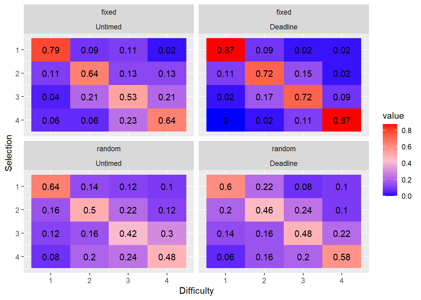
- What is the proportion of easy, medium, hard, and very hard tasks selected first, second, third or fourth?
We first compute the marginal distribution of the ranks of each of the tasks; in other words, what are the proportions of the ranks of each task in each rank position. These matrices indicate the proportions of responses for each difficulty level which were chosen first, second, third, or fourth, respectively. The matrix from a dataset in which choice is always optimal would have ones on the diagonal and zeros on the off-diagonal.
| Version | Author | Date |
|---|---|---|
| 22ddfa1 | knowlabUnimelb | 2025-07-29 |
- Do the marginal distributions differ from uniformity?
We tested whether the marginal distributions were different from uniformally random selection using the fact that the mean rank is distributed according to a \(\chi^2\) distribution with the following test-statistic: \[\chi^2 = \frac{12N}{k(k+1)}\sum_{j=1}^k \left(m_j - \frac{k+1}{2} \right)^2\] see (Marden, 1995).
condition phase chi2 df p1 fixed_location_delay untimed 67.67 3 0 2 fixed_location_delay deadline 108.52 3 0 3 random_location_delay untimed 37.80 3 0 4 random_location_delay deadline 43.85 3 0 It is evident at a glance that the ordering of choices is more optimal when the locations are fixed; that is, the proportions on the diagonal are higher. When the locations are fixed, choice order becomes more optimal under a deadline. By contrast, when locations are random, responding becomes less optimal under a deadline. This likely reflects the additional costs of having to search for the appropriate task to complete. This search is minimised in the fixed location condition.
- How optimal were responses?
| Version | Author | Date |
|---|---|---|
| 22ddfa1 | knowlabUnimelb | 2025-07-29 |
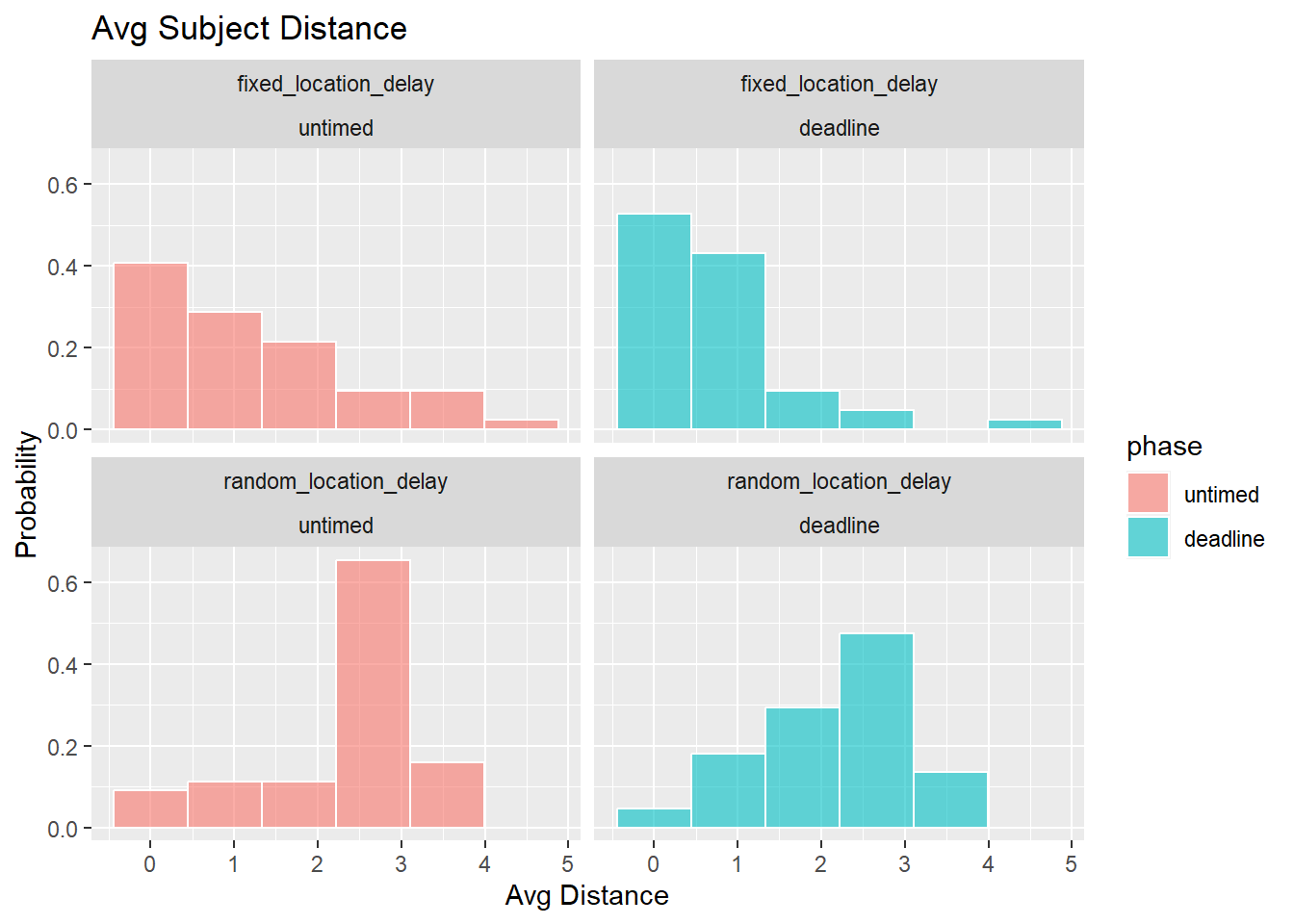
The next analysis computed the distance between the selected order and the optimal order (easiest to very hard for that trial), which ranges between 0 (perfect match) and 6 (maximally distant), for 4 options.
What we want is the distance of the selected options from the optimal solutions, which is the edit distance (or number of discordant pairs) between orders. However, because a participant may run out of time, there may be missing values. To handle these values, for each trial, we find the orders which partially match the selected order and compute three the average distance of those possible orders and the optimal solution (avg_distance).
The following figure compares the avg_distance between the fixed difficulty and random difficulty conditions as a function of deadline condition and phase. For each of these measures, lower values reflect respones which are closer to optimal.
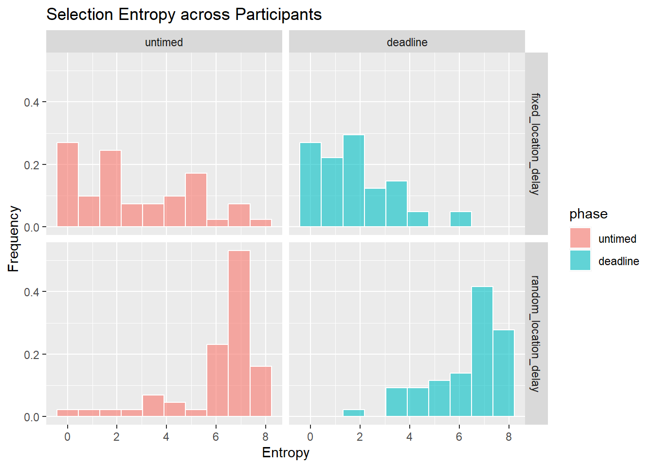
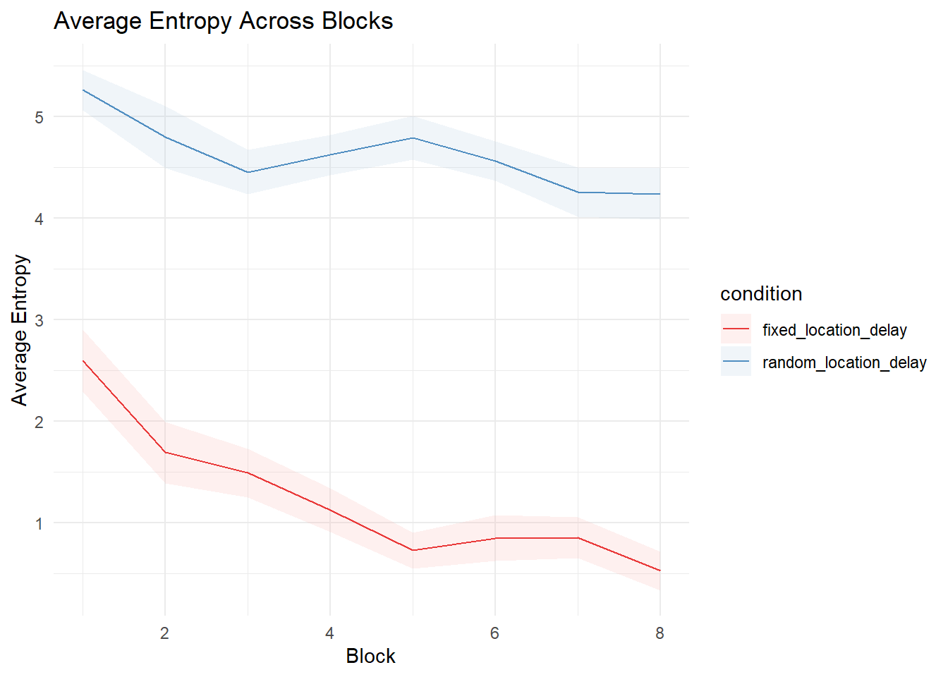
Stability of selections
| Version | Author | Date |
|---|---|---|
| 22ddfa1 | knowlabUnimelb | 2025-07-29 |
| Version | Author | Date |
|---|---|---|
| 22ddfa1 | knowlabUnimelb | 2025-07-29 |
Selection Choice RTs
| condition | phase | mrt_sel1 | mrt_sel2 | mrt_sel3 | mrt_sel4 |
|---|---|---|---|---|---|
| fixed_location_delay | deadline | 640.55 | 695.17 | 687.69 | 648.82 |
| fixed_location_delay | untimed | 1465.35 | 1340.32 | 1138.35 | 1052.31 |
| random_location_delay | deadline | 932.94 | 852.82 | 754.05 | 648.95 |
| random_location_delay | untimed | 1753.56 | 1477.17 | 1238.61 | 1071.91 |
REPEATED MEASURES ANOVA
Within Subjects Effects
────────────────────────────────────────────────────────────────────────────────────────────────────────────────
Sum of Squares df Mean Square F p η²-p
────────────────────────────────────────────────────────────────────────────────────────────────────────────────
Phase 6.006038e+7 1 6.006038e+7 238.46740425 < .0000001
0.7237967
Phase:condition 7271.572 1 7271.572 0.02887149 0.8654533 0.0003172
Residual 2.291925e+7 91 251859.901
Selection 1.026232e+7 3 3420773.448 46.80488882 < .0000001
0.3396461
Selection:condition 1721657.481 3 573885.827 7.85221902 0.0000481
0.0794339
Residual 1.995243e+7 273 73085.815
Phase:Selection 5435913.904 3 1811971.301 33.16867265 < .0000001
0.2671259
Phase:Selection:condition 16804.463 3 5601.488 0.10253689 0.9585170
0.0011255
Residual 1.491372e+7 273 54628.996
────────────────────────────────────────────────────────────────────────────────────────────────────────────────
Note. Type 3 Sums of Squares
Between Subjects Effects
──────────────────────────────────────────────────────────────────────────────────────────
Sum of Squares df Mean Square F p η²-p
──────────────────────────────────────────────────────────────────────────────────────────
condition 2108528 1 2108528.3 3.964749 0.0494615 0.0417497
Residual 4.839552e+7 91 531818.9
──────────────────────────────────────────────────────────────────────────────────────────
Note. Type 3 Sums of Squares
ASSUMPTIONS
Tests of Sphericity
───────────────────────────────────────────────────────────────────────────────────────────
Mauchly’s W p Greenhouse-Geisser ε Huynh-Feldt ε
───────────────────────────────────────────────────────────────────────────────────────────
Phase 1.0000000 NaN ᵃ 1.0000000 1.0000000
Selection 0.5473246 < .0000001 0.7313212 0.7501166
Phase:Selection 0.6875964 0.0000029 0.8305354 0.8557673
───────────────────────────────────────────────────────────────────────────────────────────
ᵃ The repeated measures has only two levels. The assumption of
sphericity is always met when the repeated measures has only two
levels.
Homogeneity of Variances Test (Levene’s)
───────────────────────────────────────────────────────── F df1 df2
p
───────────────────────────────────────────────────────── rt1_untimed
2.8647870 1 91 0.0939589
rt2_untimed 0.2607482 1 91 0.6108431
rt3_untimed 2.7707445 1 91 0.0994412
rt4_untimed 0.2886261 1 91 0.5924135
rt1_deadline 10.7284863 1 91 0.0014934
rt2_deadline 0.1544672 1 91 0.6952216
rt3_deadline 2.0923006 1 91 0.1514787
rt4_deadline 3.0166981 1 91 0.0857949
─────────────────────────────────────────────────────────
Selection model
We can treat each task selection as a probabilistic choice given by a Luce’s choice rule (Luce, 1959), where each task is represented by some strength, \(\nu\). The probability of selecting task \(i_j\) from set \(S = \{i_1, i_2, ..., i_J \}\), where J is the number of tasks, is:
\[p\left(i_j |S \right) = \frac{\nu_{i_j}}{\sum_{i \in S} \nu_{i}}. \]
Plackett (1975) generalised this model to explain the distribution over a sequence of choices (i.e., ranks). In this case, after each choice, the choice set is reduce by one (i.e., sampling without replacement). This probability of observing a specific selection order, \(i_1 \succ ... \succ i_J\) is:
\[p\left(i_j |A \right) = \prod_{j=1}^J \frac{\nu_{i_j}}{\sum_{i \in A_j} \nu_{i}}, \]
where \(A_j\) is the current choice set.
sessionInfo()R version 4.3.1 (2023-06-16 ucrt)
Platform: x86_64-w64-mingw32/x64 (64-bit)
Running under: Windows 10 x64 (build 19045)
Matrix products: default
locale:
[1] LC_COLLATE=English_Australia.utf8 LC_CTYPE=English_Australia.utf8
[3] LC_MONETARY=English_Australia.utf8 LC_NUMERIC=C
[5] LC_TIME=English_Australia.utf8
time zone: Australia/Sydney
tzcode source: internal
attached base packages:
[1] stats4 grid stats graphics grDevices utils datasets
[8] methods base
other attached packages:
[1] statmod_1.5.0 betareg_3.2-0 jmv_2.4.9 pmr_1.2.5.1
[5] jpeg_0.1-10 rstatix_0.7.2 lmerTest_3.1-3 lme4_1.1-34
[9] Matrix_1.6-1.1 png_0.1-8 reshape2_1.4.4 knitr_1.44
[13] english_1.2-6 gtools_3.9.4 DescTools_0.99.50 lubridate_1.9.3
[17] forcats_1.0.0 stringr_1.5.0 dplyr_1.1.3 purrr_1.0.2
[21] readr_2.1.4 tidyr_1.3.0 tibble_3.2.1 ggplot2_3.4.3
[25] tidyverse_2.0.0 workflowr_1.7.1
loaded via a namespace (and not attached):
[1] gld_2.6.6 sandwich_3.0-2 readxl_1.4.3
[4] rlang_1.1.1 magrittr_2.0.3 multcomp_1.4-25
[7] git2r_0.32.0 e1071_1.7-13 compiler_4.3.1
[10] flexmix_2.3-19 getPass_0.2-2 callr_3.7.3
[13] vctrs_0.6.3 pkgconfig_2.0.3 fastmap_1.1.1
[16] backports_1.4.1 labeling_0.4.3 utf8_1.2.3
[19] promises_1.2.1 rmarkdown_2.25 tzdb_0.4.0
[22] ps_1.7.5 nloptr_2.0.3 modeltools_0.2-23
[25] xfun_0.40 cachem_1.0.8 jsonlite_1.8.7
[28] later_1.3.1 afex_1.3-0 parallel_4.3.1
[31] broom_1.0.5 R6_2.5.1 RColorBrewer_1.1-3
[34] bslib_0.5.1 stringi_1.7.12 car_3.1-2
[37] boot_1.3-28.1 estimability_1.4.1 lmtest_0.9-40
[40] jquerylib_0.1.4 cellranger_1.1.0 numDeriv_2016.8-1.1
[43] Rcpp_1.0.11 zoo_1.8-12 base64enc_0.1-3
[46] nnet_7.3-19 httpuv_1.6.11 splines_4.3.1
[49] timechange_0.2.0 tidyselect_1.2.0 rstudioapi_0.15.0
[52] abind_1.4-5 yaml_2.3.7 codetools_0.2-19
[55] processx_3.8.2 lattice_0.21-8 plyr_1.8.9
[58] withr_2.5.1 coda_0.19-4 evaluate_0.22
[61] survival_3.5-5 proxy_0.4-27 pillar_1.9.0
[64] carData_3.0-5 whisker_0.4.1 generics_0.1.3
[67] rprojroot_2.0.3 hms_1.1.3 munsell_0.5.0
[70] scales_1.2.1 rootSolve_1.8.2.4 minqa_1.2.6
[73] xtable_1.8-4 jmvcore_2.4.7 class_7.3-22
[76] glue_1.6.2 emmeans_1.8.8 lmom_3.0
[79] tools_4.3.1 data.table_1.14.8 Exact_3.2
[82] fs_1.6.3 mvtnorm_1.2-3 colorspace_2.1-0
[85] nlme_3.1-162 Formula_1.2-5 cli_3.6.1
[88] fansi_1.0.4 expm_0.999-7 gtable_0.3.4
[91] sass_0.4.7 digest_0.6.33 TH.data_1.1-2
[94] farver_2.1.1 htmltools_0.5.6 lifecycle_1.0.3
[97] httr_1.4.7 MASS_7.3-60