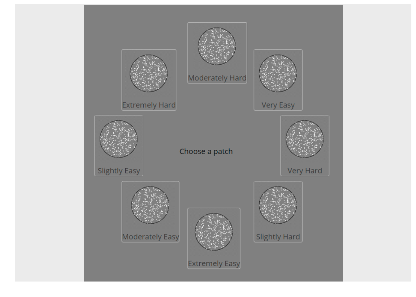
Experiment 4: RDK Direction Judgement, 8 Tasks, 500 msec Error Penalty
knowlabUnimelb
2020-10-29
Last updated: 2025-07-31
Checks: 7 0
Knit directory: SCHEDULING/
This reproducible R Markdown analysis was created with workflowr (version 1.7.1). The Checks tab describes the reproducibility checks that were applied when the results were created. The Past versions tab lists the development history.
Great! Since the R Markdown file has been committed to the Git repository, you know the exact version of the code that produced these results.
Great job! The global environment was empty. Objects defined in the global environment can affect the analysis in your R Markdown file in unknown ways. For reproduciblity it’s best to always run the code in an empty environment.
The command set.seed(20221107) was run prior to running
the code in the R Markdown file. Setting a seed ensures that any results
that rely on randomness, e.g. subsampling or permutations, are
reproducible.
Great job! Recording the operating system, R version, and package versions is critical for reproducibility.
Nice! There were no cached chunks for this analysis, so you can be confident that you successfully produced the results during this run.
Great job! Using relative paths to the files within your workflowr project makes it easier to run your code on other machines.
Great! You are using Git for version control. Tracking code development and connecting the code version to the results is critical for reproducibility.
The results in this page were generated with repository version 336572e. See the Past versions tab to see a history of the changes made to the R Markdown and HTML files.
Note that you need to be careful to ensure that all relevant files for
the analysis have been committed to Git prior to generating the results
(you can use wflow_publish or
wflow_git_commit). workflowr only checks the R Markdown
file, but you know if there are other scripts or data files that it
depends on. Below is the status of the Git repository when the results
were generated:
Ignored files:
    Ignored:    .Rhistory
    Ignored:    .Rproj.user/
    Ignored:    analysis/patch_selection.png
    Ignored:    analysis/patch_selection_8.png
    Ignored:    analysis/patch_selection_avg.png
    Ignored:    analysis/site_libs/

Untracked files:
    Untracked:  analysis/Notes.txt
    Untracked:  analysis/additional_scripts.R
    Untracked:  analysis/analysis_2025_deadlines.Rmd
    Untracked:  analysis/analysis_2025_dynamicNoise_fixed.Rmd
    Untracked:  analysis/analysis_exp10_preemption.Rmd
    Untracked:  analysis/analysis_exp10_preemption1and2.Rmd
    Untracked:  analysis/analysis_exp10b_preemption-pareto.Rmd
    Untracked:  analysis/analysis_exp11_facesInNoise.Rmd
    Untracked:  analysis/analysis_exp11_facesInNoise_EW.Rmd
    Untracked:  analysis/analysis_exp11_facesInNoise_EW_v2.Rmd
    Untracked:  analysis/analysis_exp12_variability.Rmd
    Untracked:  analysis/analysis_exp12_variability_cynthia.Rmd
    Untracked:  analysis/analysis_exp12_variability_cynthia_update.Rmd
    Untracked:  analysis/analysis_exp13_preemption.Rmd
    Untracked:  analysis/analysis_exp14_ASD_individual_differences.Rmd
    Untracked:  analysis/analysis_exp9_preselection.Rmd
    Untracked:  analysis/analysis_exp9_preselection1and2.Rmd
    Untracked:  analysis/analysis_exp9_select-then-complete.Rmd
    Untracked:  analysis/anovaData/
    Untracked:  analysis/archive/
    Untracked:  analysis/correlation_test.m
    Untracked:  analysis/fd_pl.rds
    Untracked:  analysis/fu_pl.rds
    Untracked:  analysis/instructions_for_honours_students.txt
    Untracked:  analysis/joyPlot.m
    Untracked:  analysis/joyPlot.zip
    Untracked:  analysis/joyPlot/
    Untracked:  analysis/loadData.m
    Untracked:  analysis/mstrfind.m
    Untracked:  analysis/plotDistanceByTrials.m
    Untracked:  analysis/prereg/
    Untracked:  analysis/reward rate analysis.docx
    Untracked:  analysis/rewardRate.jpg
    Untracked:  analysis/scheduling_analysis_functions.R
    Untracked:  analysis/temp/
    Untracked:  analysis/toAnalyse/
    Untracked:  analysis/wflow_code_string.txt
    Untracked:  code/AUTSIMQ/
    Untracked:  code/DYNAMICNOISE/
    Untracked:  code/FACESINNOISE/
    Untracked:  code/Notes on how the scheduling jsPsych code works.txt
    Untracked:  code/PREEMPT/
    Untracked:  code/PREPLAN/
    Untracked:  code/SCHEDULEPIX/
    Untracked:  code/SCHEDULEPIX_UON/
    Untracked:  code/SCHEDULERDK/
    Untracked:  code/SCHEDULERDK_UON/
    Untracked:  code/SCHEDULE_REWARD/
    Untracked:  code/SCHEDULE_TYPING/
    Untracked:  code/SMALL_N_LETTERNOISE/
    Untracked:  code/TRAIN_PREEMPT/
    Untracked:  code/TRAIN_VARYING_DEADLINES/
    Untracked:  code/autism_quotient.txt
    Untracked:  data/2020_exp1_rdk_data.csv
    Untracked:  data/2020_exp2_rdk_data.csv
    Untracked:  data/2021_exp2b_rdk_data_avgtime.csv
    Untracked:  data/2021_exp3a_rdk_data_dynamic.csv
    Untracked:  data/2021_exp3b_rdk_data_dynamic_highlight.csv
    Untracked:  data/2021_exp3c_rdk_data_dynamic_shortdotlife.csv
    Untracked:  data/2022_exp4_rdk_data_8tasks.csv
    Untracked:  data/2023-exp10-preemption-pareto.csv
    Untracked:  data/2023-exp10-preemption-selections.csv
    Untracked:  data/2023-exp10-preemption.csv
    Untracked:  data/2023-exp11-facesInNoise-unlabelledCondition.csv
    Untracked:  data/2023-exp11-facesInNoise.csv
    Untracked:  data/2023-exp9-preplan.csv
    Untracked:  data/2023-exp9-select-then-complete.csv
    Untracked:  data/2023_AQdata.csv
    Untracked:  data/2024-exp12-variability.csv
    Untracked:  data/2024-exp12-variability_v2.csv
    Untracked:  data/2024-exp12-variability_v3.csv
    Untracked:  data/2024-exp13-preemption.csv
    Untracked:  data/2024-exp13-preemption_v2.csv
    Untracked:  data/2024-scheduling-data.csv
    Untracked:  data/2024_data_rdk_select_first_AQcorrelation_update.csv
    Untracked:  data/2024_data_typing_train_variability.csv
    Untracked:  data/2025_data_dynamic_noise_fixed_locations.csv
    Untracked:  data/2025_data_typing_train_deadlines_exp1rates.csv
    Untracked:  data/2025_data_typing_train_variability_fulldataset.csv
    Untracked:  data/ASRSscoring.csv
    Untracked:  data/OLIFEscoring.csv
    Untracked:  data/OLIFEscoring_v0.csv
    Untracked:  data/POLYscoring.csv
    Untracked:  data/SQL query.txt
    Untracked:  data/archive/
    Untracked:  data/create_database.sql
    Untracked:  data/dataToAnalyse/
    Untracked:  data/data_dictionary_deadlines.csv
    Untracked:  data/data_dictionary_dynamic_noise.csv
    Untracked:  data/data_dictionary_facesInNoise.csv
    Untracked:  data/data_dictionary_preemption.csv
    Untracked:  data/data_dictionary_preplan.csv
    Untracked:  data/data_dictionary_select_then_complete.csv
    Untracked:  data/data_dictionary_variability.csv
    Untracked:  data/exp6a_typing_exponential.xlsx
    Untracked:  data/exp6b_typing_linear.xlsx
    Untracked:  data/exp8a_typing_no_reward_data_selections.csv
    Untracked:  data/rawdata_incEmails/
    Untracked:  data/selections/
    Untracked:  data/sona data/
    Untracked:  data/summaryFiles/
    Untracked:  data/temp_AQcorrelationReplication/
    Untracked:  spatial_pdist.Rdata

Unstaged changes:
    Modified:   analysis/analysis_exp1_labelled_nodelay.Rmd
    Modified:   analysis/analysis_exp2a_labelled_delay.Rmd
    Modified:   analysis/analysis_exp7e_rdk_reward_points.Rmd
    Modified:   analysis/analysis_exp8a_typing_no_reward.Rmd
    Deleted:    analysis/prereg.Rmd
    Deleted:    analysis/prereg_v2.Rmd
    Deleted:    analysis/prereg_v3.Rmd
    Deleted:    analysis/prereg_v6_AQcorrelation.Rmd
    Modified:   data/README.md
    Modified:   data/data_dictionary.csv
    Modified:   data/data_dictionary_8.csv
    Modified:   data/data_dictionary_avgTime.csv
    Modified:   data/data_dictionary_ruby.csv
    Modified:   data/data_dictionary_shortdotlife.csv
    Deleted:    data/exp1_rdk_data.csv
    Deleted:    data/exp2_rdk_data.csv
    Deleted:    data/exp2b_rdk_data_avgtime.csv
    Deleted:    data/exp3a_rdk_data_dynamic.csv
    Deleted:    data/exp3b_rdk_data_dynamic_highlight.csv
    Deleted:    data/exp3c_rdk_data_dynamic_shortdotlife.csv
    Deleted:    data/exp4_rdk_data_8tasks.csv
Note that any generated files, e.g. HTML, png, CSS, etc., are not included in this status report because it is ok for generated content to have uncommitted changes.
These are the previous versions of the repository in which changes were
made to the R Markdown
(analysis/analysis_exp4_8tasks_labelled_delay.Rmd) and HTML
(docs/analysis_exp4_8tasks_labelled_delay.html) files. If
you’ve configured a remote Git repository (see
?wflow_git_remote), click on the hyperlinks in the table
below to view the files as they were in that past version.
| File | Version | Author | Date | Message |
|---|---|---|---|---|
| Rmd | 336572e | knowlabUnimelb | 2025-07-31 | Update analysis code to use shared file repo |
| html | 2e6ecdf | knowlabUnimelb | 2022-11-09 | Build site. |
| Rmd | 67e1aac | knowlabUnimelb | 2022-11-09 | Publish data and analysis files |
Daniel R. Little1 and Ami Eidels2 1 The University of Melbourne, 2 The University of Newcastle
Data Analysis
We first summarize performance by answering the following questions:
Task completions
- How many tasks are completed on average?
| phase | mean | sd |
|---|---|---|
| untimed | 7.67 | 1.14 |
| deadline | 7.16 | 1.23 |
ONE SAMPLE T-TEST
One Sample T-Test
──────────────────────────────────────────────────────────────────────────────────────────────
Statistic df p Effect Size
──────────────────────────────────────────────────────────────────────────────────────────────
deadline Student’s t 27.02124 46.00000 < .0000001 Cohen’s d
3.941453
──────────────────────────────────────────────────────────────────────────────────────────────
Note. Hₐ μ ≠ 0
Normality Test (Shapiro-Wilk)
────────────────────────────────────── W p
────────────────────────────────────── deadline 0.7977782
0.0000014
────────────────────────────────────── Note. A low p-value suggests a
violation of the assumption of normality
Descriptives
──────────────────────────────────────────────────────────────────── N
Mean Median SD SE
────────────────────────────────────────────────────────────────────
deadline 47 3.159574 3.400000 0.8016269 0.1169293
────────────────────────────────────────────────────────────────────
RDK performance
- What was the average completion time and accuracy of the easy, medium, hard, and very hard tasks?
| Version | Author | Date |
|---|---|---|
| 2e6ecdf | knowlabUnimelb | 2022-11-09 |
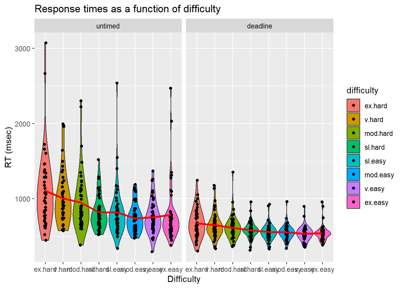
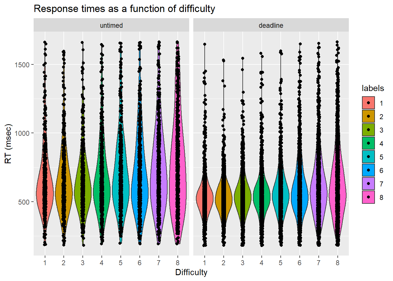
We further broke down RTs by condition, deadline, and difficulty.
Reward Rate
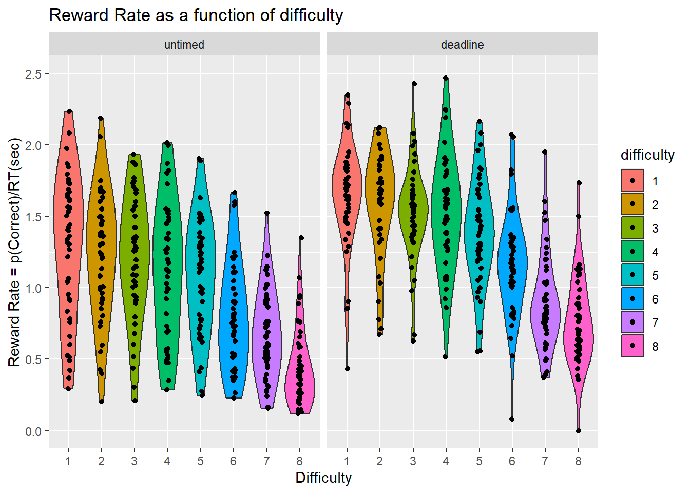
| name[none] | ss[none] | df[none] | ms[none] | F[none] | p[none] | partEta[none] | |
|---|---|---|---|---|---|---|---|
| “Phase” | Phase | 22.406 | 1 | 22.406 | 142.603 | 0.00 | 0.756 |
| [“Phase”,“.RES”] | Residual | 7.228 | 46 | 0.157 | NA | NA | NA |
| “Difficulty” | Difficulty | 69.571 | 7 | 9.939 | 107.471 | 0.00 | 0.700 |
| [“Difficulty”,“.RES”] | Residual | 29.778 | 322 | 0.092 | NA | NA | NA |
| [“Phase”,“Difficulty”] | Phase:Difficulty | 0.573 | 7 | 0.082 | 1.186 | 0.31 | 0.025 |
| [“Phase”,“Difficulty”,“.RES”] | Residual | 22.219 | 322 | 0.069 | NA | NA | NA |
| name | ss | df | ms | F | p | partEta | |
|---|---|---|---|---|---|---|---|
| “Residual” | Residual | 48.205 | 46 | 1.048 | NA | NA | NA |
Optimality in each condition
Having now established that the RDK’s are ordered in accuracy, difficulty, and reward rate, it is clear that the task set presented to each subject has an optimal solution, ordered from easiest to most difficult. We now ask:
- What is the proportion of easy, medium, hard, and very hard tasks selected first, second, third or fourth?
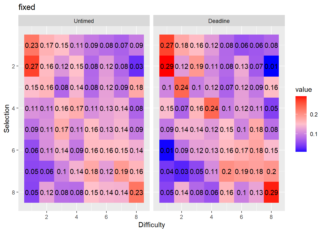
- Do the marginal distributions differ from uniformity?
We tested whether the marginal distributions were different from uniformally random selection using the fact that the mean rank is distributed according to a \(\chi^2\) distribution with the following test-statistic: \[\chi^2 = \frac{12N}{k(k+1)}\sum_{j=1}^k \left(m_j - \frac{k+1}{2} \right)^2\] see (Marden, 1995).
| condition | phase | chi2 | df | p |
|---|---|---|---|---|
| fixed | untimed | 264.06 | 3 | 0 |
| fixed | deadline | 1367.28 | 3 | 0 |
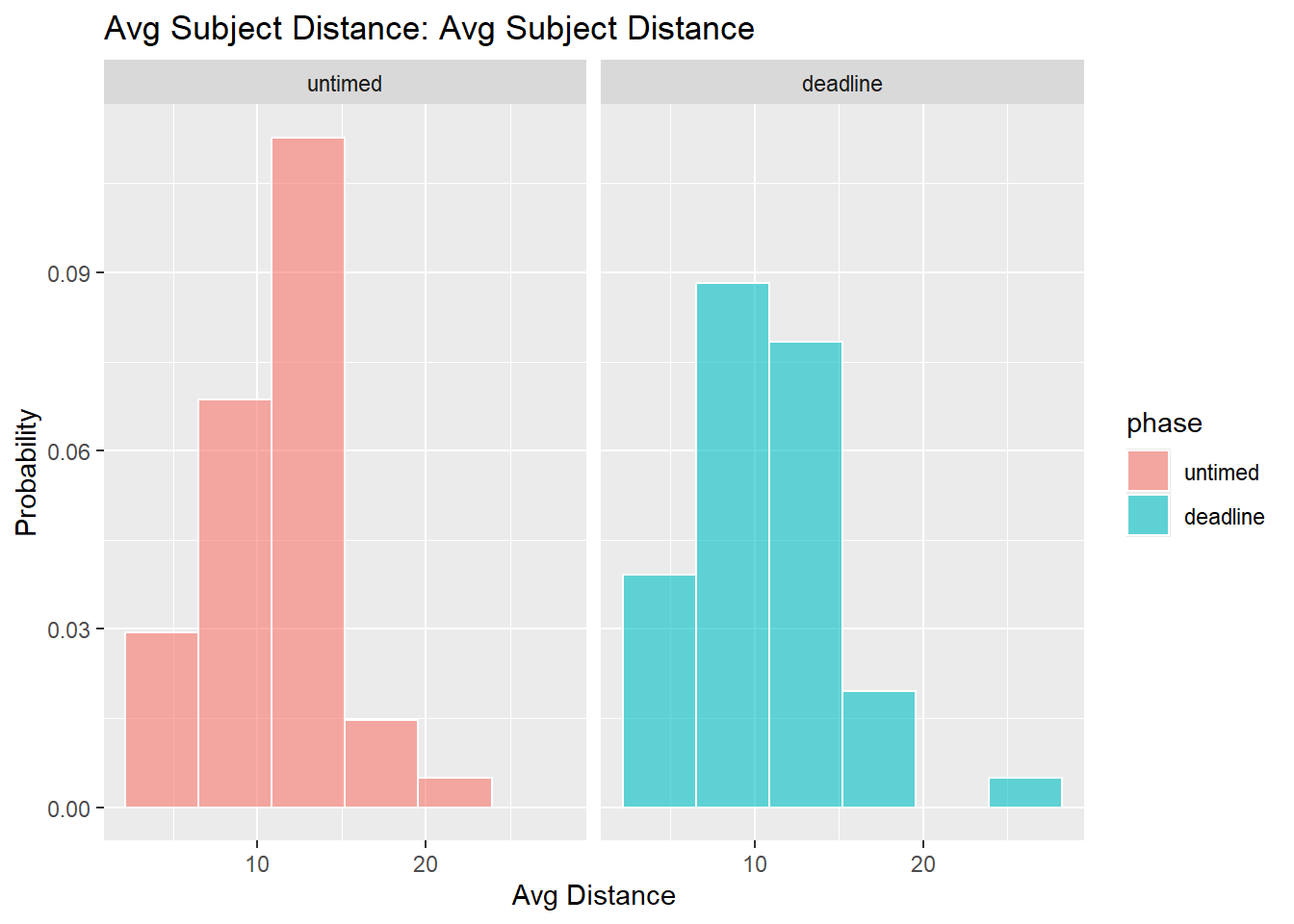
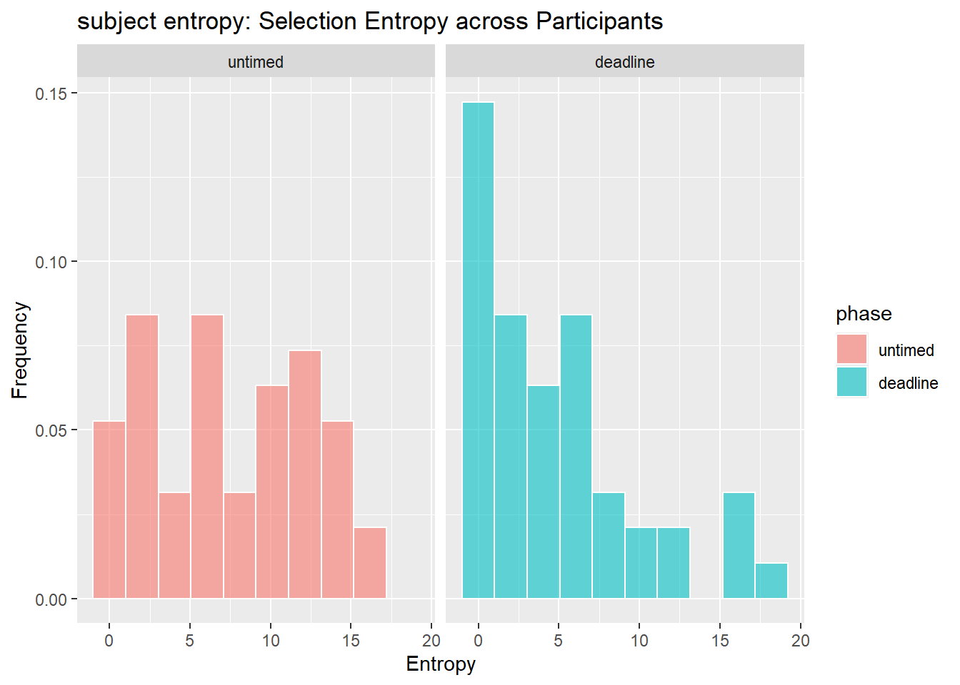
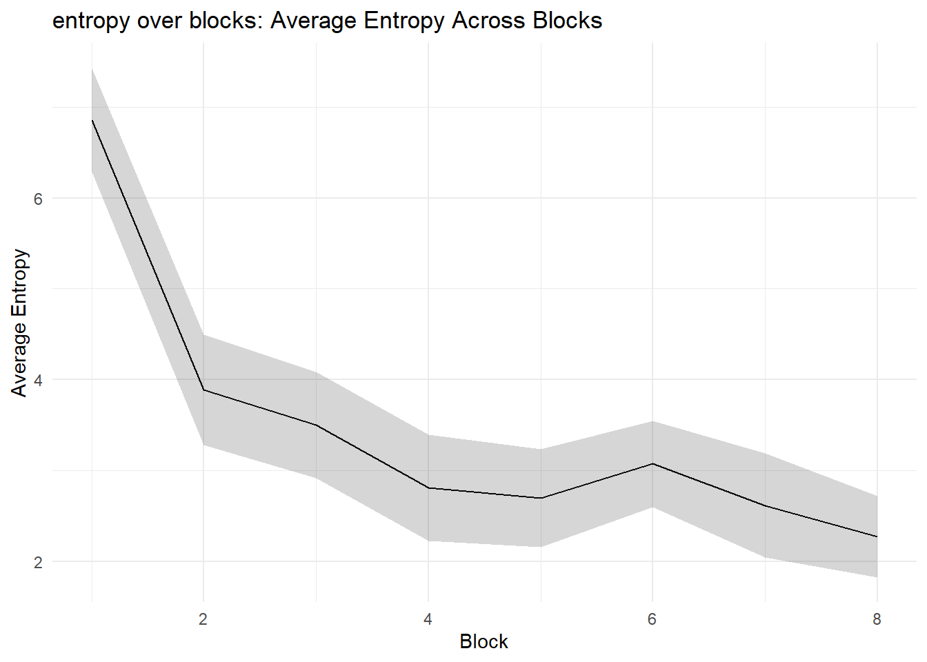
Stability of selections
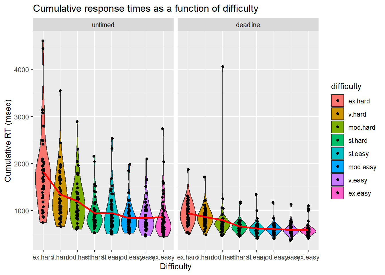
Selection Choice RTs
| condition | phase | mrt_selrt_1 | mrt_selrt_2 | mrt_selrt_3 | mrt_selrt_4 | mrt_selrt_5 | mrt_selrt_6 | mrt_selrt_7 | mrt_selrt_8 |
|---|---|---|---|---|---|---|---|---|---|
| fixed_location_8_delay | deadline | 670.81 | 471.13 | 478.95 | 500.13 | 514.87 | 503.44 | 497.05 | 490.26 |
| fixed_location_8_delay | untimed | 1528.76 | 912.24 | 796.52 | 768.89 | 735.85 | 690.94 | 681.19 | 732.26 |
REPEATED MEASURES ANOVA
Within Subjects Effects
───────────────────────────────────────────────────────────────────────────────────────────────────
Sum of Squares df Mean Square F p η²-p
───────────────────────────────────────────────────────────────────────────────────────────────────
Phase 2.083516e+7 1 2.083516e+7 228.40502 < .0000001 0.8323646
Residual 4196132 46 91220.25
Selection 1.417607e+7 3 4725357.92 109.54658 < .0000001
0.7042687
Residual 5952713 138 43135.60
Phase:Selection 5077782 3 1692594.05 61.20413 < .0000001
0.5709121
Residual 3816376 138 27654.90
───────────────────────────────────────────────────────────────────────────────────────────────────
Note. Type 3 Sums of Squares
Between Subjects Effects
──────────────────────────────────────────────────────────────────────────────────
Sum of Squares df Mean Square F p η²-p
──────────────────────────────────────────────────────────────────────────────────
Residual 1.273978e+7 46 276951.6
──────────────────────────────────────────────────────────────────────────────────
Note. Type 3 Sums of Squares
ASSUMPTIONS
Tests of Sphericity
───────────────────────────────────────────────────────────────────────────────────────────
Mauchly’s W p Greenhouse-Geisser ε Huynh-Feldt ε
───────────────────────────────────────────────────────────────────────────────────────────
Phase ᵃ 1.0000000 NaN 1.0000000 1.0000000
Selection 0.1249106 < .0000001 0.4556628 0.4648910
Phase:Selection 0.2608010 < .0000001 0.5362752 0.5527735
───────────────────────────────────────────────────────────────────────────────────────────
ᵃ The repeated measures has only two levels. The assumption of
sphericity is always met when the repeated measures has only two
levels.
Homogeneity of Variances Test (Levene’s)
──────────────────────────────────────────────────── F df1 df2 p
──────────────────────────────────────────────────── rt1_untimed NaN
ᵃ
rt2_untimed NaN ᵃ
rt3_untimed NaN ᵃ
rt4_untimed NaN ᵃ
rt1_deadline NaN ᵃ
rt2_deadline NaN ᵃ
rt3_deadline NaN ᵃ
rt4_deadline NaN ᵃ
──────────────────────────────────────────────────── ᵃ As there are no
between subjects factors specified this assumption is always met.
Selection model
We can treat each task selection as a probabilistic choice given by a Luce’s choice rule (Luce, 1959), where each task is represented by some strength, \(\nu\). The probability of selecting task \(i_j\) from set \(S = \left{i_1, i_2, ..., i_J \right}\), where J is the number of tasks, is:
\[p\left(i_j |S \right) = \frac{\nu_{i_j}}{\sum_{i \in S} \nu_{i}} \].
Plackett (1975) generalised this model to explain the distribution over a sequence of choices (i.e., ranks). In this case, after each choice, the choice set is reduce by one (i.e., sampling without replacement). This probability of observing a specific selection order, \(i_1 \succ ... \succ i_J\) is:
\[p\left(i_j |A \right) = \prod_{j=1}^J \frac{\nu_{i_j}}{\sum_{i \in A_j} \nu_{i}} \],
where \(A_j\) is the current choice set.
sessionInfo()R version 4.4.2 (2024-10-31 ucrt)
Platform: x86_64-w64-mingw32/x64
Running under: Windows 11 x64 (build 26100)
Matrix products: default
locale:
[1] LC_COLLATE=English_Australia.utf8 LC_CTYPE=English_Australia.utf8
[3] LC_MONETARY=English_Australia.utf8 LC_NUMERIC=C
[5] LC_TIME=English_Australia.utf8
time zone: Australia/Sydney
tzcode source: internal
attached base packages:
[1] stats4 grid stats graphics grDevices utils datasets
[8] methods base
other attached packages:
[1] statmod_1.5.0 betareg_3.2-3 jmv_2.7.0 pmr_1.2.5.1
[5] jpeg_0.1-11 rstatix_0.7.2 lmerTest_3.1-3 lme4_1.1-37
[9] Matrix_1.7-1 png_0.1-8 reshape2_1.4.4 knitr_1.49
[13] english_1.2-6 gtools_3.9.5 DescTools_0.99.60 lubridate_1.9.4
[17] forcats_1.0.0 stringr_1.5.1 dplyr_1.1.4 purrr_1.1.0
[21] readr_2.1.5 tidyr_1.3.1 tibble_3.3.0 ggplot2_3.5.2
[25] tidyverse_2.0.0 workflowr_1.7.1
loaded via a namespace (and not attached):
[1] mnormt_2.1.1 Rdpack_2.6.4 gld_2.6.7
[4] sandwich_3.1-1 readxl_1.4.5 rlang_1.1.4
[7] magrittr_2.0.3 multcomp_1.4-28 git2r_0.35.0
[10] e1071_1.7-16 compiler_4.4.2 flexmix_2.3-20
[13] getPass_0.2-4 callr_3.7.6 vctrs_0.6.5
[16] pkgconfig_2.0.3 fastmap_1.2.0 backports_1.5.0
[19] labeling_0.4.3 promises_1.3.0 rmarkdown_2.29
[22] tzdb_0.5.0 haven_2.5.5 ps_1.8.1
[25] nloptr_2.2.1 modeltools_0.2-24 xfun_0.49
[28] cachem_1.1.0 jsonlite_1.8.9 later_1.3.2
[31] afex_1.4-1 psych_2.5.6 parallel_4.4.2
[34] broom_1.0.9 R6_2.5.1 bslib_0.8.0
[37] stringi_1.8.4 RColorBrewer_1.1-3 car_3.1-3
[40] boot_1.3-31 estimability_1.5.1 lmtest_0.9-40
[43] jquerylib_0.1.4 cellranger_1.1.0 numDeriv_2016.8-1.1
[46] Rcpp_1.0.13-1 zoo_1.8-14 base64enc_0.1-3
[49] nnet_7.3-19 httpuv_1.6.15 splines_4.4.2
[52] timechange_0.3.0 tidyselect_1.2.1 rstudioapi_0.17.1
[55] abind_1.4-8 yaml_2.3.10 codetools_0.2-20
[58] processx_3.8.4 lattice_0.22-6 plyr_1.8.9
[61] withr_3.0.2 coda_0.19-4.1 evaluate_1.0.1
[64] survival_3.7-0 proxy_0.4-27 pillar_1.11.0
[67] carData_3.0-5 whisker_0.4.1 reformulas_0.4.1
[70] generics_0.1.4 rprojroot_2.0.4 hms_1.1.3
[73] scales_1.4.0 rootSolve_1.8.2.4 minqa_1.2.8
[76] jmvcore_2.6.3 class_7.3-22 glue_1.8.0
[79] emmeans_1.11.2 lmom_3.2 tools_4.4.2
[82] data.table_1.17.8 Exact_3.3 fs_1.6.5
[85] mvtnorm_1.3-3 rbibutils_2.3 nlme_3.1-166
[88] Formula_1.2-5 cli_3.6.3 expm_1.0-0
[91] gtable_0.3.6 sass_0.4.9 digest_0.6.37
[94] TH.data_1.1-3 farver_2.1.2 htmltools_0.5.8.1
[97] lifecycle_1.0.4 httr_1.4.7 MASS_7.3-61